Understanding potential wells
To think about potential wells, we often imagine little beads rolling on the plot of the potential well (as a wire) under gravity without friction. How precise is this analogy?
Let’s consider a system with one degree of freedom being described by \(\ddot x = f(x), \; x \in \mathbb{R}\) with kinetic energy \(T = \frac{1}{2} \dot x^2\) and potential energy \(U(x) = - \int_{x_0}^x f(\xi) d \xi\). Alternatively we could write
\[\ddot x = -\frac{dU}{dx}\]Potential wells in reality
Suppose we have some function \(U(x)\). Imagine a bead of mass 1 moving along a wire \(\{(x, U(x)) \,\vert\, x \in \mathbb{R}\}\) under gravity with zero fiction. The lagrangian of the system is hence \(\frac{1}{2} (\dot x^2 + \dot y^2) - gy\). Imposing the constraint \(y = U(x)\), the lagrangian is now
\[\begin{align*} L&=\frac{1}{2} (\dot x^2 + \dot y^2) - gy\\ &= \frac{1}{2} \bigg(\dot x^2 + \dot x^2 \bigg(\frac{dU}{dx}\bigg)^2\bigg) - g U(x) \\ &= \frac{1}{2} \dot x^2 \bigg(1 + \bigg(\frac{dU}{dx}\bigg)^2\bigg)- gU(x) \end{align*}\]The Euler-Lagrange equation would now be
\[\begin{align*} 0&= \frac{d}{dt}\bigg(\frac{\partial L}{\partial {\dot x}} \bigg) - \frac{\partial L}{\partial x} \\ &= \frac{d}{dt}\bigg[\dot x \bigg(1 + \bigg(\frac{dU}{dx}\bigg)^2\bigg)\bigg] \\ &\phantom{= } -\bigg[ \frac{1}{2}\dot x^2\frac{d}{dx}\bigg(\bigg(\frac{dU}{dx}\bigg)^2\bigg) - g \frac{dU}{dx}\bigg] \\ &= \ddot x \bigg(1 + \bigg(\frac{dU}{dx}\bigg)^2\bigg) + \dot x \bigg(\dot x \frac{d}{dx}\bigg(\bigg(\frac{dU}{dx}\bigg)^2\bigg)\bigg) \\ &\phantom{= }-\bigg[ \frac{1}{2}\dot x^2\frac{d}{dx}\bigg(\bigg(\frac{dU}{dx}\bigg)^2\bigg)- g \frac{dU}{dx}\bigg] \\ &= \ddot x \bigg(1 + \bigg(\frac{dU}{dx}\bigg)^2\bigg) + \dot x \bigg(\dot x \times 2 \frac{dU}{dx} \frac{d^2U}{dx^2}\bigg) \\ &\phantom{= }-\bigg[ \frac{1}{2}\dot x^2\times 2 \frac{dU}{dx} \frac{d^2U}{dx^2}- g \frac{dU}{dx}\bigg] \\ &= \ddot x \bigg(1 + \bigg(\frac{dU}{dx}\bigg)^2\bigg) + \frac{dU}{dx} \bigg(\dot x^2\frac{d^2U}{dx^2} + g\bigg) \end{align*}\]Hence
\[\ddot x = \frac{-\frac{dU}{dx}}{1+(\frac{dU}{dx})^2} \bigg(g + \dot x^2 \frac{d^2 U}{ dx^2} \bigg)\]This isn’t particularly illuminating. Let’s understand the above term by term.
First Term: \(\frac{-\frac{dU}{dx}}{1+(\frac{dU}{dx})^2} g\)
Let \(\theta\) be the normal angle of \(U(x)\) to the \(x\)-axis, then we could write \(-\frac{dU}{dx}\) as \(\tan \theta\). Now we would have \(\frac{-\frac{dU}{dx}}{1+(\frac{dU}{dx})^2} = \frac{- \tan \theta}{1 + \tan^2 \theta} = -\sin \theta \cos \theta\). As such we have
\[\frac{-\frac{dU}{dx}}{1+(\frac{dU}{dx})^2} g = \cos \theta \times (-g \sin \theta)\]This could be thought of as the horizontal component of the normal component of gravitational acceleration.
Second Term: \(\frac{-\frac{dU}{dx}}{1+(\frac{dU}{dx})^2}\dot x^2 \frac{d^2 U}{ dx^2}\)
We would like to connect the second derivative of \(U(x)\) with its curvature as follows.
\[\begin{align*} &\dot x^2 \frac{-\frac{dU}{dx}}{1+(\frac{dU}{dx})^2} \frac{d^2 U}{ dx^2} \\ &= \frac{\dot x^2 + \dot y^2}{1 + (\frac{dU}{dx})^2} \times \bigg(-\frac{dU}{dx} \sqrt{1+\bigg(\frac{dU}{dx}\bigg)^2}\bigg) \times \frac{\frac{d^2 U}{dx^2}}{(1+(\frac{dU}{dx})^2)^{3/2}} \\ &= v^2 \times - \cos \theta \times \kappa \\ &= \cos \theta \times (- v^2/r) \end{align*}\]where \(v\) is the magnitude of velocity, \(\kappa\) is the signed curvature and \(r\) is the signed radius of curvature. \(\frac{v^2}{r}\) could be understood as the centripetal acceleration, \(a_c\), necessary to keep the bead on the wire. \(a_c\) is positive if the curve opens upwards and negative if the curve opens downwards.
Combining the two terms, we have
\[\ddot x = \cos \theta ( - g \sin \theta - a_c)\]\(-g \sin \theta - a_c\) could be thought of as the magnitude of the net acceleration on the bead. The multiplier \(\cos \theta\) nets us the horizontal component.
Comparing the two potentials
Setting \(g = 1\), if \(a_c \ll 1\) (e.g. initial velocity is \(0\) or the curvature of \(U(x)\) is close to \(0\)) then \(\ddot x \approx - \cos \theta \sin \theta\). This is strikingly similar to the case of the abstract potential well for low \(\theta\) where \(\ddot x = - \frac{dU}{dx} = \tan \theta\). We could see this by plotting \(-\tan \theta\) in red and \(-\sin \theta \cos \theta\) in blue.
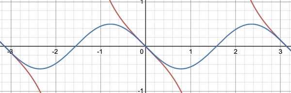
For the abstract potential wall, the acceleration it could capture is unbounded. For the potential well “in reality”, the acceleration is bounded by one half of gravitational acceleration.
Pendulum potential
If \(U(x) = -\cos x\), for an abstract potential well we could plot the phase diagram as follows: (x-axis is \(x\) while y-axis is \(\dot x\))
\[\begin{align*} \dot x &= y \\ \dot y &= -\sin x \end{align*}\]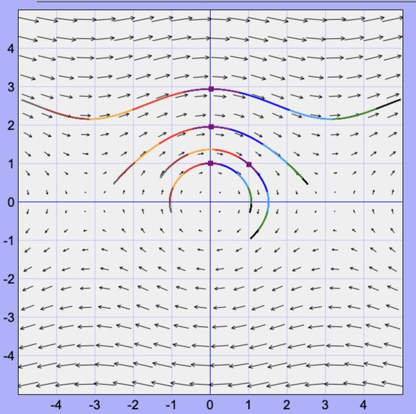
For a potential well “in reality” we have
\[\begin{align*} \dot x &= y \\ \dot y &=\frac{-\sin x}{1 + \sin^2 x} \big( 1 + y^2 \cos x \big) \end{align*}\]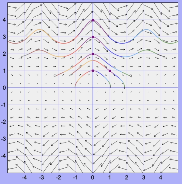
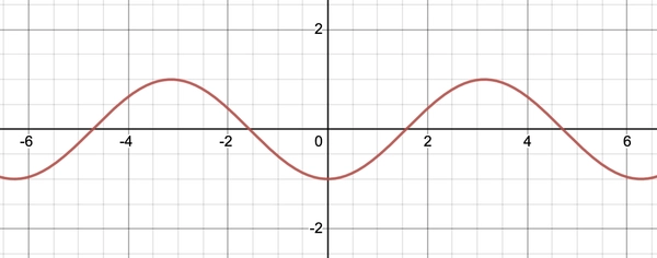
There are now local minimums of \(\dot x\) around \(x=\pi/2\), that’s because the curvature of \(-\cos x\) changes sign and the vertical velocity starts converting back into horizontal velocity due to the constraint force. The peaks of \(\dot x\) at \(x=\pi\) are also lowered as there’s less gravitational potential energy. Below is a plot of \(U(x) = - \cos x\) for reference.
Quadractic potential
If \(U(x) = x^2\), for an abstract potential well we could plot the phase diagram as follows: (x-axis is \(x\) while y-axis is \(\dot x\))
\[\begin{align*} \dot x &= y \\ \dot y &= -2x \end{align*}\]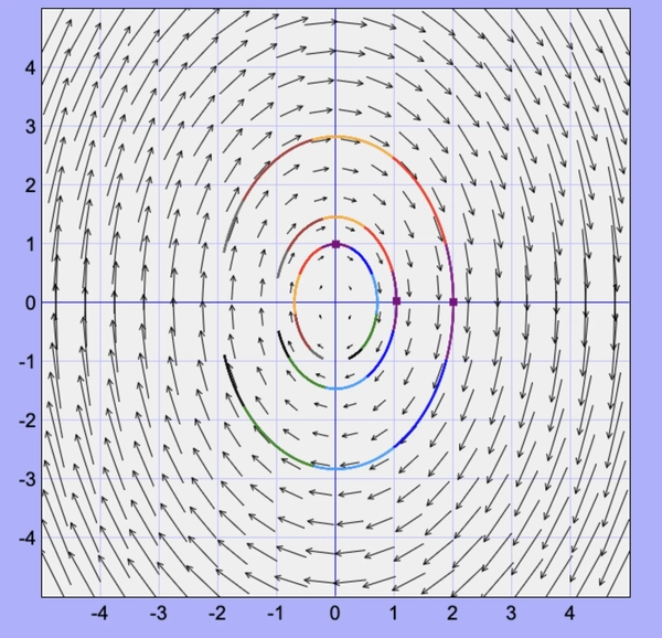
For a potential well “in reality” we have
\[\begin{align*} \dot x &= y \\ \dot y &= \frac{-2x}{1+4x^2}( 1 + 2 y^2 ) \end{align*}\]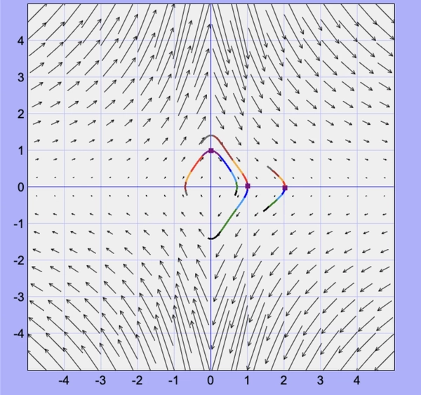
Acknowledgments
Thanks to a phase plane plotter by Ariel Barton.