A physical interepertation of trigonometric substitution
Below are some proofs by pictures of the derivatives of trigonometric functions, which would hopefully enable greater geometric understanding. They also give rise to a alternate physical understanding of why integration by substitution works. Some of these ideas come from a stack exchange post. We’d focus on one example, the tangent function.
Tangent function
We could visualise the derivative of the tangent function \(x=\tan \theta\) as follows.
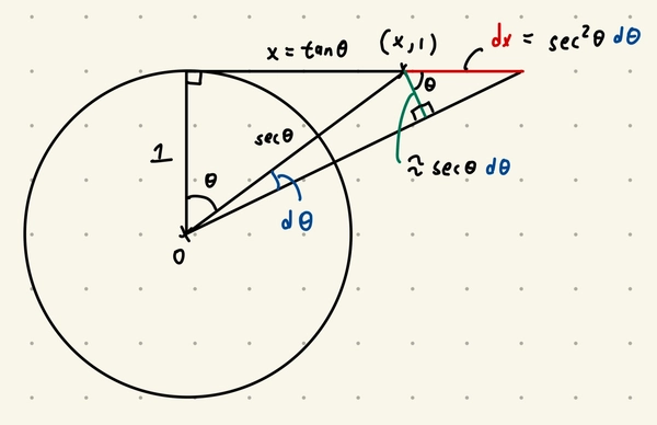
Motivated by the above, given any integral \(\int_0^{L} f(x, 1, \sqrt{x^2+1}) \, dx\), we could interept it as the line integral \(\int_\gamma f(x, y, \sqrt{x^2+y^2})\,dt\) w.r.t the curve \(\gamma = \{(t,1) \;\vert\;t \in [0, L]\}\). The relationship between the two integrals could be summarised as follows.
\[\begin{align*} x &\iff \text{Horizontal distance } x = \tan \theta, \\ 1 &\iff \text{Vertical distance } y = 1, \\ \sqrt{x^2+1} &\iff \text{Radial distance } \sqrt{x^2+y^2} = \sec \theta. \end{align*}\]In practice, we use the following
\[\int_0^L f(x, 1, \sqrt{x^2+1}) \, dx = \int_0^{\arctan L} f(\tan \theta, 1, \sec \theta) \sec^2(\theta) \, d\theta.\]This gives rise to an interesting physical interepertation of integration by substitution. If we had a infinitely long rod with a uniform mass desnity of \(1\) at \(y=1\), the above states that if we are only interested at the gravitational field at the origin, we could’ve replaced the rod with a circular wire with mass density \(\cos^2 \theta\).
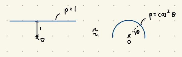
In essence, we’ve collapsed the degree of freedom of distance into mass density.
This argument holds locally / even if the rod wasn’t infintely long. We could also clearly extend this argument to arbtiary mass distributions.
Going further
One could find visualizations of the derivatives of sine / cosine here.