Graph sketching techniques
We’d cover techniques of sketching graphs of compositions of functions (i.e. \(f(g(x))\)) and when one could approximate graphs with simpler ones.
Preliminaries
Here’s a quick run-down on things you can do generally
- Finding x, y-intercepts
- Finding asymptotes (in a general sense)
- Finding symmetries (odd / even / reflectional / translational / periodicity)
Make sure to not have these techniques take hold of your mathematical thinking. These techniques should serve your mathematical thinking not the other way round. Always keep an open mind to simpler / intuitive arguments.
I however hold a dim view on the following
- Find the derivative / critical points
- Find the second derivative / inflection points
Finding them is certainly important. However usually you’d end up with even more complicated formulae than you started off – the effort to results ratio is often quite low. Asymptotic and symmetric properties also often greatly limit the behaviour of critical / inflection points.
Compositions
Whenever you’re asked to sketch the graph of some composition \(f(g(x))\), it’s very useful to sketch the graph of \(f(x)\) and \(g(x)\) seperatedly and “chase the plots”. For example, to sketch \(\sin (\frac{1}{x})\), you could first sketch \(\sin x\) and \(\frac{1}{x}\).
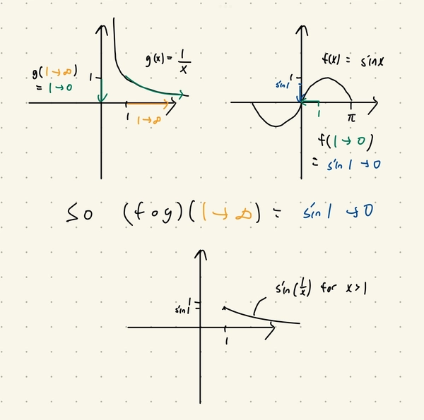
If one is uncomfortable with the use of arrows we could replace them with intervals. The use of arrows only let us better understand if the function is increasing or decreasing.
Approximations
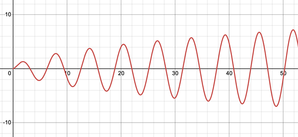
To sketch the graph \(f(x)g(x)\) around \(x=p\), sometimes it looks like scaled versions of the graphs of \(f(x)\) or \(g(x)\). For example in the plot of \(\sqrt{x}\sin x\) below, you notice that when \(x\) is large it almost looks identical to the plot of \(\sin x\) scaled up by a constant factor. Why is that?
We could understand this by looking at the linear approximation of \(f(x)g(x)\). We observe that
\[\begin{align*} f(x)g(x) &\approx f(p)g(p) + (f(x)g(x))'|_{x=p}(x-p) \\ &= f(p)g(p) + (f'(p)g(p) + f(p)g'(p))(x-p). \end{align*}\]If \(f'(p) \approx 0\) i.e. when \(p\) is nearly a critical point of \(f\), then
\[\begin{align*} f(x)g(x) &\approx f(p)g(p) + f(p)g'(p)(x-p) \\ &= f(p)\times[g(p) + g'(p)(x-p)] \\ &\approx f(p)g(x) \end{align*}\]so we can sketch \(f(x)g(x)\) as \(f(p)g(x)\) around \(x=p\).
Back to our previous example, as the slope of \(\sqrt{x}\) tends to \(0\) as \(x\) increases, we have \(\sqrt{x}\sin x\) looking like \(\sqrt{p} \sin x\) around \(x=p\) when \(p\) is large.
Generally this idea works as long as \(f(p)g'(p) \gg f'(p)g(p)\).
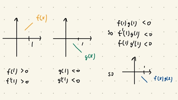
Related to this, if \(f'(p)g(p)\) and \(f(p)g'(p)\) have the same sign then you would know the sign of \(f'(p)g(p) + f(p)g'(p)\) which tells you the slope of the tangent line of \(f(x)g(x)\) at \(x=p\). This isn’t as unlikely as it seems, see the example below.
Quick-fire Round
- Make sure your graphs are neatly drawn (axis, labels).
- Try to split complicated functions into multiple parts and sketch them seperatedly.
- Your intercepts / critical points / inflection points do not to have to be exact, as long as the relative size of the values you calculate is preserved.
- Given \(f(x)\), if \(f'(x)\) is continuous then \(f\) is increasing or decreasing in between critical points (supposing that \(f, f'\) is defined in between the critical points). This is generally very helpful if you already know where the critical points are.