A circle and a hyperbola living in one plot
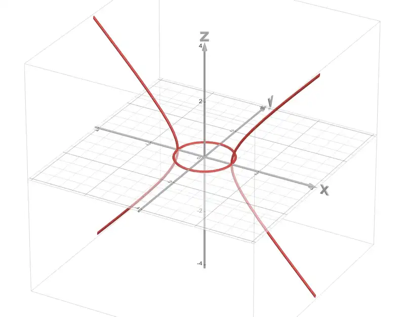
We will see that the 3D plot of \(x^2 + (y + zi)^2 = 1\), where \(x\), \(y\), \(z\) are real and \(i\) is the imaginary unit, contains both a circle and a hyperbola. This visualization sheds light on the complex eigenvalues of real matrices.
Let’s start by expanding the equation \(x^2+(y+zi)^2 = 1\) and separating it into real and imaginary parts. We get:
\[\begin{align*} &\text{Real Part:} &x^2 + y^2 - z^2 &= 1, \\ &\text{Imaginary Part:} &yz &= 0. \end{align*}\]The condition \(yz=0\) splits into two cases:
\[\begin{align*} \text{Case 1: }y&=0 \text{ and so } x^2-z^2 = 1\\ \text{Case 2: }z&=0 \text{ and so } x^2+y^2 = 1 \end{align*}\]Case 1 nets us a hyperbola in the \(xz\)-plane. Case 2 nets us a unit circle in the \(xy\)-plane.
You can check out the plot at desmos.
Eigenvalues and dynamical systems
Why does this matter beyond the visuals? These kinds of plots often appears when studying the (complex) eigenvalues of a real matrix that depends on a real parameter. For example, consider the matrix
\[M(\mu) = \begin{bmatrix} 0 & 1+\mu \\ 1-\mu & 0 \end{bmatrix}\]for real \(\mu\).
The eigenvalues \(\lambda\) of \(M\) satisify the equation \(\mu^2 + \lambda^2 = 1.\) Letting \(\mu = x\) and \(\lambda = y+zi\) recovers the plot of \(x^2 + (y+iz)^2 = 1.\)
From the geometry of the plot, we can immediately read off the eigenvalue behavior:
\[\begin{align*} \mu < -1&: M(\mu) \text{ complex conjugate eigenvalues} \\ \mu = -1&: M(\mu) \text{ repeated eigenvalue } \lambda = 0 \\ -1 < \mu < 1&: M(\mu) \text{ one }+\text{ve and one }-\text{ve real eigenvalue} \\ \mu = 1&: M(\mu) \text{ repated eigenvalue } \lambda = 0 \\ \mu > 1&: M(\mu) \text{ complex conjugate eigenvalues} \end{align*}\]More examples
Consider the matrix
\[M(\mu) = \begin{bmatrix} 1 & \mu \\ 1 & 1 \end{bmatrix}\]and think about its eigenvalues as a function of \(\mu\).
When \(\mu=1\), \(M(\mu)\) is degenerate and so has a zero eigenvalue. When \(\mu=0\), \(M(\mu)\) is a shear matrix with only one eigenvalue \(\lambda = 1\). As shear matrices live on the boundary of diagonalisable and non-diagonalisable matrices, we can reasonably further guess that if \(\mu<0\) then \(M(\mu)\) has complex conjugate eigenvalues and if \(\mu>0\) then \(M(\mu)\) has real eigenvalues.
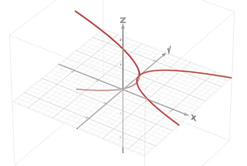
Concretely, considering the eigenvalue equation \(\lambda^2 - 2\lambda + (1-\mu) = 0\) and letting \(\mu=x\) and \(\lambda=y+zi\) and re-arranging terms we get
\[\left((y+zi)-1\right)^2=x.\]By splitting into real parts and imaginary parts and re-arranging terms we get
\[\begin{align*} &\text{Real Part:} &(y-1)^2 - z^2 &= x, \\ &\text{Imaginary Part:} &(y-1)z &= 0. \end{align*}\]Again we have two cases
\[\begin{align*} \text{Case 1: }y&=1 \text{ and so } -z^2 = x\\ \text{Case 2: }z&=0 \text{ and so } (y-1)^2 = 0 \end{align*}\]Case 1 nets us a parabola in the \(xz\)-plane while Case 2 nets us a parabola in the \(xy\)-plane. Finally, we arrive at the plot.
You can create these sort of plots for any other 2 by 2 matrix that depends on one real parameter using a desmos calculator I made.