Visualising bifurications
Given a one-dimensional dynamical system \(\dot x = f(x, \mu)\) where \(\mu\) is some parameter, one could plot \(f\) as a function of \(x, \mu\) in 3D. The zeros of \(f\) are the critical points. If at the critical point \((x_0, \mu_0)\) we have \(\tfrac{\partial f}{\partial x}\vert_{(x_0, \mu_0)} < 0\), then the critical point is stable.
Doing so enables greater geometric reasoning about bifurications, e.g. why saddle-node bifurications are robust but transcritical and pitchfork bifurications are not.
Examples
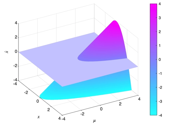
\(\dot x = \mu - x^2\) could be plotted as follows
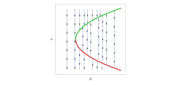
which corresponds to the classical bifurication diagram
We can see that as \(\tfrac{\partial \dot x}{\partial x} = -2x\), all critical points with \(x>0\) are stable while all critical points with \(x<0\) are unstable.
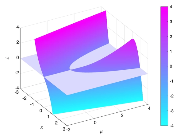
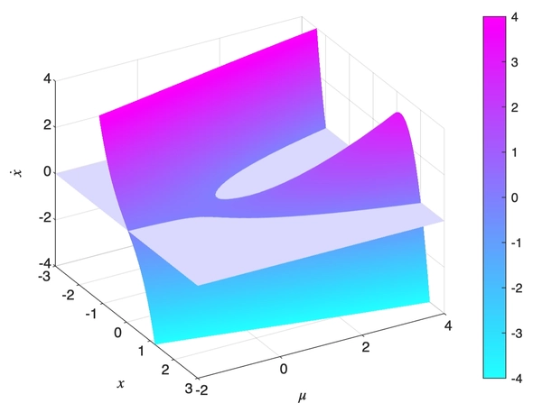
\(\dot x = \mu x - x^3\) could be plotted as follows
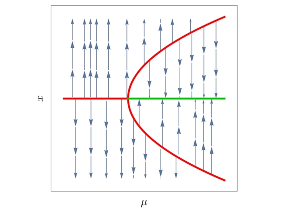
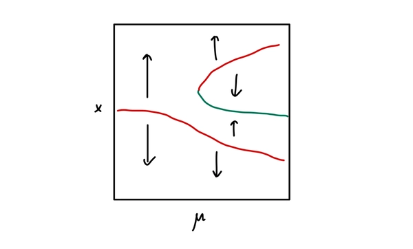
which corresponds to the classical bifurication diagram
We could see that the above is not robust by considering \(\dot x = \mu x - x^3 + \epsilon\) for some small \(\epsilon > 0\). Below we’ve plotted what would happen if \(\epsilon = 0.1\). Compared to our previous plot, we could imagine it as the grey water level moving down by \(\epsilon\) with the terrain unchanged.
Now we would have the classical bifurication diagram as follows
These techniques generalises well to other simple bifurications. Here’s the MATLAB code for you to try out yourself!
[X,Y] = meshgrid(-5:0.1:5,-5:0.1:5);

Z = zeros(size(X));
surf(X,Y,Z,'FaceAlpha',0.3); hold on
Z = X.*Y-X.*X.*X+0.1*ones(size(X));
surf(X,Y,Z); hold on

xlabel('$x$','interpreter','latex')
ylabel('$\mu$','interpreter','latex')
zlabel('$\dot{x}$', 'interpreter','latex')

xlim([-3 3])
ylim([-2 4])
zlim([-4 4])
clim([-4 4])
view([60 35])
colormap('cool')
colorbar
shading interp