Three ways of thinking about matrix multiplication
I’ve found thinking about matrix multiplication in the following three ways to be exceptionally helpful, especially at understanding why elementary row operations are on the left and why elementary column operations are on the right.
We shall use 3 by 3 matrices as the motivating example throughout, although it can be generalised to higher dimensions. Let’s introduce some notation first.
Notation
Let \(\mathbf{A}\) be a 3 by 3 matrix
\[\mathbf{A} = \left[\begin{array}{ccc} a_{11} & a_{12} & a_{13} \\ a_{21} & a_{22} & a_{23} \\ a_{31} & a_{32} & a_{33} \end{array}\right]\]For \(i, j \in \{1, 2, 3\}\), we define its row and column vectors as follows
\[\mathbf{A}_i = \left[\begin{array}{c} a_{i1} & a_{i2} & a_{i3} \end{array}\right]\] \[\mathbf{A}^j= \left[\begin{array}{c} a_{1j} \\ a_{2j} \\ a_{3j} \end{array}\right]\]Using this notation, we can write
\[\mathbf{A} = \left[\begin{array}{ccc} \mathbf{A}^1 & \mathbf{A}^2 & \mathbf{A}^3 \end{array}\right] = \left[\begin{array}{c} \mathbf{A}_1 \\ \mathbf{A}_2 \\ \mathbf{A}_3 \end{array}\right]\]Standard Interpretation
Let \(\mathbf{B}\) be another 3 by 3 matrix. We usually define the product of \(\mathbf{A}\) and \(\mathbf{B}\) to be a 3 by 3 matrix with coefficients
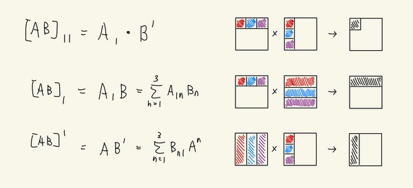
\[[\mathbf{AB}]_{ij} = \sum_{k=1}^3 a_{ik} b_{kj}\]Alternatively we could view the above as the dot product of row vectors of \(\mathbf{A}\) and column vectors of \(\mathbf{B}\). I.e. we have
\[[\mathbf{AB}]_{ij} = \mathbf{A}_i \cdot \mathbf{B}^j\]I.e.
\[\begin{align*}\mathbf{AB} &= \left[\begin{array}{c} \mathbf{A}_1 \cdot \mathbf{B}^1 & \mathbf{A}_1 \cdot \mathbf{B}^2 & \mathbf{A}_1 \cdot \mathbf{B}^3\\ \mathbf{A}_2 \cdot \mathbf{B}^1 & \mathbf{A}_2 \cdot \mathbf{B}^2 & \mathbf{A}_2 \cdot \mathbf{B}^3\\ \mathbf{A}_3 \cdot \mathbf{B}^1 & \mathbf{A}_3 \cdot \mathbf{B}^2 & \mathbf{A}_3 \cdot \mathbf{B}^3 \end{array}\right]\\ &=\left[\begin{array}{c} \mathbf{A}_1 \\ \mathbf{A}_2 \\ \mathbf{A}_3 \end{array}\right]\left[\begin{array}{ccc} \mathbf{B}^1 & \mathbf{B}^2 & \mathbf{B}^3 \end{array}\right]\end{align*}\]Row Interpretation
Alternatively we can think about the row vectors of \(\mathbf{A}\mathbf{B}\). From the above we could see that the \(i\)-th row vector of \(\mathbf{A}\mathbf{B}\) is
\[\begin{align*} [\mathbf{A}\mathbf{B}]_i&=\left[\begin{array}{ccc}\mathbf{A}_i \cdot \mathbf{B}^1 & \mathbf{A}_i \cdot \mathbf{B}^2 & \mathbf{A}_i \cdot \mathbf{B}^3\end{array}\right] \\ &= \mathbf{A}_i \left[\begin{array}{ccc} \mathbf{B}^1 & \mathbf{B}^2 & \mathbf{B}^3 \end{array}\right] \\ &= \mathbf{A}_i \mathbf{B} \end{align*}\]Column Interpretation
Similarly we can consider the column vectors of \(\mathbf{A}\mathbf{B}\). From the above we could see that the \(j\)-th column vector of \(\mathbf{A}\mathbf{B}\) is
\[\begin{align*} [\mathbf{A}\mathbf{B}]^j&=\left[\begin{array}{c} \mathbf{A}_1 \cdot \mathbf{B}^j \\ \mathbf{A}_2 \cdot \mathbf{B}^j\\ \mathbf{A}_3 \cdot \mathbf{B}^j \end{array}\right] \\ &= \left[\begin{array}{c} \mathbf{A}_1 \\ \mathbf{A}_2 \\ \mathbf{A}_3 \end{array}\right] \mathbf{B}^j \\ &= \mathbf{A} \mathbf{B}^j \end{align*}\]Proof by picture

Exercises
Here are some exercises